Hopfield Networks are models of content addressable memory. In other words, they are dynamical systems designed to encode $N$ arbitrary strings and then converge to a point of perfect recall of any one of these strings if stimulated with any noised version of one of these strings. The usual textbook presentation on Hopfield networks begins by presenting the dynamical system without any motivation and only then going on to study its properties.

Here, I build a hopfield network from the bottom up. I begin with a motivating question that leads to a Bayesian formulation of the problem. Gradient based optimization yields an expression remarkably similar to the actual Hopfield network. By taking a first order taylor approximation of the derived dynamical system, I arrive at the true update rule for Hopfield nets. I then study (currently a work in progress) the dynamical properties of this Hopfield network.

The present article follows in the spirit of my previous train of articles, ending with The Dynamics of Gradient Descent in Linear Least Squares Regression.

Perhaps in a sequel article I will try to extend the Hopfield network, which currently operates on binary signals, to continuous valued inputs as well as to translation and scale invariance.

Deriving a Dynamical System

Implementing content addressable memory as a dynamical systems necessitates an ansatz equation, i.e. some initial symbolic structure to play around with. (As much as the field would like its neuronal models to be structure free, the only way to get there is by making simplifying assumptions and introducing structure.).

Let there be $N$ unique binary strings of length $K$ indexed by $\mu$, $\mathbf{x}^\mu$, which can be observed with some bits randomly flipped, i.e. signal noise.

Input Strings

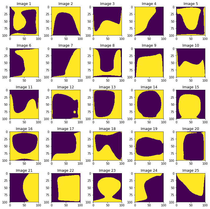
Such observations are initially sampled from a uniform distribution over binary strings and then this string is permuted by sampling from a noise distribution. Observations will be denoted by the random variable $\mathbf{X}$. In particular, a single bit in random observation $X_j$ is kept with probability $1-p$ and flipped with probability $p$. In particular, let the permutative process be interpreted as a random variable $\zeta$ defined over the binary sample space $\Omega = {-1, 1}$ (The author originally tried ${0,1}$ as a sample space but came to a point where this definition made some terms very difficult to deal with analytically. As such, the paper will follow the convention of using the range of the $\text{sgn}$ function as its binary digits).Now, $\zeta_j \sim \text{Bernoulli}(p)$

such that

$$X_j = x_j\zeta_j$$

It follows that it is in fact the case $X_j = x_j$ with probability $1-p$ and $X_j=-x_j$ with probability $p$.

Henceforth will be derived a dynamical system to converge upon the most likely true signal given some noisy observation of it, as defined in (1). Specifically, the system will be represented by $T$ units, each denoted by $z_j$ which evolve over time. These units in the system are initialized with a random sample from the observation distribution.

$$z_{j}(0) \sim \text{Bernoulli}(p)$$

The network’s prediction $\mathbf{z}$ of the true denoised signal $\mathbf{x}$ can be optimized by maximizing the likelihood that it is in fact the true signal. This means solving the program

$$\arg \max\limits_{\mathbf{z_j}}\mathcal{P}(\mathbf{z}_j(0))$$

First, I define a uniform distribution over the set of true signals.

$$\mathcal{P}(\mathbf{x}) = \frac{1}{N}$$

Next, I write a distribution for the likelihood of observing any noised signal given the true signal.

$$\mathcal{P}(\mathbf{\tilde{x}} \mid \mathbf{x}) = \alpha^{H_\mu }\beta^{T-H_\mu} \\$$

where $\alpha =\frac{p}{1-p}$, $\beta = 1-p$ and $H_\mu$ is the number of pairwise different bits betIen the $\mu$th true signal $\mathbf{x}^\mu$ and the current estimate of the true signal $z_j$,

$$H_\mu =\sum\limits_{j=1}^T x_j\wedge z_j\\$$

in which $a \wedge b$ is the logical $\text{EQUALITY}$ operator. Equation $(7)$ is merely a symbolic abstraction and is now rewritten explicitly.

$$H_\mu = \frac{1}{2} \left[ N - \sum\limits_{j=1}^T z_jx^\mu_j \right] = \frac{1}{2}\left[N- \mathbf{z}\cdot\mathbf{x}^\mu \right]$$

It is beneficial to take a moment to understand equation $(8)$. If $z_j = x_j$, i.e. the network’s prediction matches the true value, then $z_jx_j = 1$. Otherwise, $z_jx_j = -1$. Thus,

$$\sum x_jz_j = C - I$$

where $C$ is the number of correct guesses and $I$ is the number of incorrect guesses. We would like only the number of incorrect guesses, i.e. $H^\mu = I$. Observe that $C=N-I$, such that

$$\sum x_jz_j = N- 2I$$

Thus

$$\frac{1}{2}\left[ N - \sum x_j z_j = I \right]$$

The above two distributions for $\mathcal{P}(\mathbf{x})$ and $\mathcal{P}(\mathbf{z(0)} \mid \mathbf{x}) $ can be combined with Bayes rule to write an expression for total probability of any initial state $z_j(0)$. While it may be advantageous to do so, for the sake of simplicity, the present discussion will not discuss the case of adding a bayesian prior.

$$\mathcal{P}(\mathbf{z}(0)) = \sum\limits^N_{\mu=1}\mathcal{P}(\mathbf{z}(0)\mid\mathbf{x}^\mu)\mathcal{P}(\mathbf{x}^\mu)$$ $$\mathcal{P}(\mathbf{z}(0)) = \frac{\beta ^T}{N}\sum\limits^N_{\mu=1} \exp\left\{H_\mu\ln\alpha \right\} \\$$

By maximizing $(12)$, we arrive at an optimal prediction $\mathbf{z}$.

$$\frac{\partial \mathcal{P}(z_j)}{\partial z_j} = \frac{\beta^T}{N}\ln\alpha\sum\limits^N_{\mu=1} \exp\left\{H_\mu\ln\alpha \right\} \frac{\partial H_\mu}{\partial z_j}$$

From $(8)$,

$$\frac{\partial H_\mu}{\partial {z}_j} = -\frac{1}{2}x_j^\mu$$

Noting that $z_j$ is bounded to the closed interval $[-1, 1]$, I could use Lagrangian optimization to solve for

$$\frac{\partial \mathcal{P}(z_j)}{\partial z_j} = 0$$

Keeping $z_j$ in a closed interval is equivalent to saying $|z_j| = \sqrt{z_j^2} = 1$. Thus, ​
$\nabla z_j = \lambda \frac{z_j}{|z_j|}$

Because of the absolute value in the denominator, this will be really difficult to solve analytically. Do not fear. Due to the very simple bounds on $z_j$,gradient ascent is a viable solution but only if I place a nonlinear filter over each update to keep $z_j$ in line. The reason for this is because the learning equations Ire derived with the assumption that the range is bounded; I must therefore enforce this constraint in our updates because gradient descent cannot read our minds. Furthermore, it will not be necessary to perform a numerical integration $z_j:= z_j + \Delta z_j$ because I care only about the sign of $z_j$ and nothing more. As such, whether $\Delta z_j >0 $ or $\Delta z_j < 0$ is sufficient for our interests.

$$z_j:= \tanh\left\{\kappa \sum\limits^N_{\mu=1}x_j^\mu \alpha^{H_\mu} \right\}$$

where $\kappa$ is a chosen rate of convergence. If updates are to be discrete then the rule becomes very similar to the true hopfield update rule

$$z_j := \text{sgn}\left\{ \sum\limits^N_{\mu=1}x_j^\mu \alpha^{H_\mu} \right\}$$

Learning Process

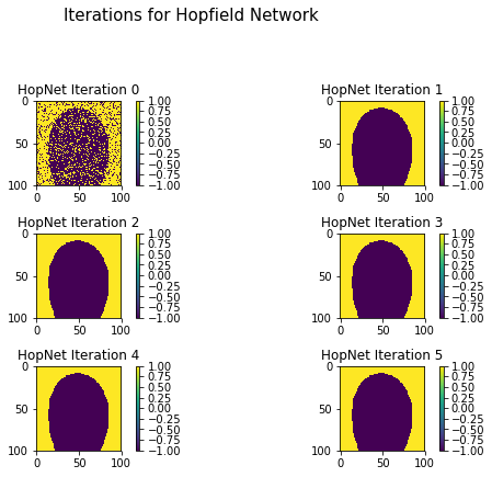
We have arrived at something very similar to the real Hopfield update rule by starting with maximum likelihood concerns. This shows that real Hopfield networks not only converge upon a solution, but onto a statistcally optimal one.

Some simulations have shown that the given Hopfield update rule actually blows up quite quickly, causing numerical overflow. Because we really only care about the magnitude of each output node and not the rate of convergence, we can linearize the given update rule by taking its taylor expansion.

Extensions

Continuous Networks

I can read your mind. The Hopfield networks we worked with here are nice and all but they are only configured on binary inputs. No fear; the networks rely on Hamming distance, which is a continuous function of its inputs. Thus, if instead of being limited to ${-1,1}$, the range $x_i$ and $z_j$ was expanded without notice to the entire interval $[-1, 1]$, continuity and monotonicity ensures everything will work as expected.

Interval Equality

The next issue we face is elitism. You see, Hopfield networks only serve those special variables that live in a very small part of the numerical world, $[-1, 1]$. Because we are so caring we need to provide equal opportunity for all noisy input signals to be reconstructed. We also have additional worries. The excluded numbers might start suing and charging discrimination. At that point, there will be boycotts, politically charged exchange of words…who knows what will happen. The entire numerical universe might just overflow. In addition, when you have really noisy crowds of numbers, 2 might take on the persona of .4, masquerade as such, infiltrate the inner circle, and rise to a position of prominance only to be unmasked. Do we really want to risk such a scandal? Of course not.

So really, what do we do?

Well, we’re using $\tanh$ already to keep the outputs bounded, so why not just use it initially to keep the inputs bounded. To do this effectively, we need to preserve the relative scale of all numbers. This is easily accomplished by Z-Scoring all input signals and then running them through a nonlinearity $\tanh$. This comes with a cherry on top for free, which is that the same network is invariant to scale by only operating on relative scale. Some tests using $\tanh$ as a bounding nonlinearity unfortunately show that $\tanh$ saturates too quickly to really preserve the relative magnitudes of all inputs. If this is a concern, it might be best to just Z-Score.

Analysis of The Hopfield Dynamical System

As a sanity check, we can confirm that equation $(18)$ does in fact converge upon the true value by working backwards. Assume $z_j \approx x^w_j =1 $. Then

$$\sum\limits^N_{\mu=1}x_j^\mu \alpha^{H_\mu} \approx x^w_j$$

For this to happen, it must be that

$$x^w_j a^{H_w} > \sum\limits_{\mu \ne w} x^\mu_j \alpha^{H_\mu}$$

This is only the case if $0< \alpha \ll 1$. Given that $\alpha = \frac{p}{1-p}$, this requires $p \ll1-p$, or that the signal to noise ratio is very high.

Conclusion

We have shown that a Hopfield-like system emerges quite naturally when you ask the same question that Hopfield did and take a maximum likelihood approach to ansIring it. where $\kappa$ is the arbitrarily chosen rate of convergence. Eventually this system will converge on the denoised signal.

I usually post my blog articles before they are finished as an incentive for me to finish them. come back later and I’ll do more in depth analysis of the stability and nuance in the Hopfield network I just derived

Supplementary Materials

The python implementation of hopfield networks used to generate the figures is located here.

Bibliography

Hancock, Edwin R., and Josef Kittler. “A Bayesian interpretation for the Hopfield network.” Neural Networks, 1993., IEEE International Conference on. IEEE, 1993.