Arguably, one of the most powerful developments in early modern applied mathematics is that of gradient descent, which is a technique for solving programs of the form

$$\arg\max _w f(w)$$

by solving a dynamical system

$$\mathbf{w}_{t+1} := \mathbf{w}+\lambda(\mathbf{w}\mid \mathbf{x}, \mathbf{y})$$

In this paper, we show in the case of a simple least-squares linear regression optimization that the chosen learning rate determines both whether the algorithm will ever converge as well as the rate of convergence itself. Furthermore, we derive a partition of the real line such that learning rates from each of these partitions results in distinct dynamics for the discrete gradient update dynamical system. We show that for only very well selected learning rates will the algorithm ever converge. That such results may be theoretically derived is an innovation in the toolkit used by those who develop and study learning algorithms. It shows that after learning rules have been derived, additional analysis must be performed to understand the asymptotic behavior and stability dynamics of the dynamical system defined by the learning rules.

Bounds on Learning Rate $\alpha$ for which Learning Converges

Suppose we have already derived the learning rules for a D dimensional regression from the normality assumption. $y = \mathbf{w} \mathbf{x}$

Also, we have removed all constants of proportionality in the learning equations for the sake of simplicity, which doesn’t change the asymptotic behavior of learning.

Let $\alpha$ be a learning rate, $\mathbf{x}$ be a $D$ by $T$ matrix, $\mathbf{y}$ a 1 by T matrix, and $\mathbf{w}$ a D dimensional row vector.

$\begin{align} \Delta w_{i,t} &= -\alpha \sum\limits^N_j (y_i-\hat{y}_j)x_j \\ &= -\alpha \sum\limits^N_j (y_i-w_jx_{ij})x_{ij}\\ &= -\alpha \mathbf{x}_i\cdot\mathbf{y}\frac{1}{N} + w_{i,t}\alpha \mathbf{x}_i\cdot\mathbf{x}_i\frac{1}{N} \end{align}$ Observe in this linear task the dynamics of each weight $w_i$ is independent of that of any other weight. We can simplify equation (2) by writing $\beta_ {i1}= - \alpha\mathbf{x_i}\cdot\mathbf{y}\frac{1}{N}$ and $\beta_{i2}=\alpha\mathbf{x}_i \cdot\mathbf{x}_i\frac{1}{N}$, such that $\Delta w_{i,t} = \beta_{i1}+\beta_{i2}w_{it}$

We would like to analyze the asymptotic behavior of this dynamical system and to do so we need an analytical expression for $w_{i,t}$. First, we will produce an update rule

$$w_{i,t+1} = \beta_{i1}+w_{it} (\beta_{i2}+1)$$

which we recognize as a one dimensional autoregressive process with an affine term. We can recursively compose equation (5) with itself, using $w_{i,0} \sim \mathcal{N}(\mu, \sigma)$ as initial conditions. This is a bit of a tedious computation that results in a closed form polynomial expression. We simplify the indices in the computation by assuming it holds for all $w_i$. Thus subscripts in the computation on $w$ refer to iterations, with dimension implied. $\begin{align} w_{0} &= w_0\\ w_{1} &= \beta_1+w_0(\beta_2+1) \\ w_2 &= \beta_1+\beta_1(\beta_2+1)+w_0(\beta_2+1)^2\\ w_3 &= \beta_1 + \beta_1(\beta_2+1)+\beta_1(\beta_2+1)^2+w_0(\beta_2+1)^3\\ w_n &=w_0(\beta_2 + 1)^n + \beta_1\sum^{n-1}_{j=0}(\beta_2+1)^j \end{align}$

This leads to somewhat of a closed form expression:

$$w_{it} = (\beta_{i2}+1)^t w_{i0}+\beta_{i1}\sum\limits^{t-1}_{j=1}(\beta_{i2}+1)^j$$

We are interested in the limit $t\to \infty$ as it relates to $\alpha$.

$$\lim\limits_{t\to\infty} \left [w_{it} = (\beta_{i2}+1)^t w_{i0}+\beta_{i1}\sum\limits^{t-1}_{j=1}(\beta_{i2}+1)^j \right] =\ ?$$

Both terms in (8) converge if $-1 < \beta_{i2}+1 < 1$. Recalling from before $\beta_{i2} =\alpha\mathbf{x_i}\cdot\mathbf{x_i}\frac{1}{N}$,

$$\begin{align} -1 < &\beta_{i2}+1 <1 \\ -1 < &\alpha\frac{\|\mathbf{x}\|^2}{N} + 1 < 1 \\ \end{align}$$

There are two cases to consider and we now go through them:

If

$$0 \le \alpha\frac{\|\mathbf{x}\|^2}{N} + 1 < 1$$

then

$$-1 \le \alpha\frac{\|\mathbf{x}\|^2}{N} < 0$$

Thus

$$-1 \le \frac{\alpha}{N}|\mathbf{x}|^2 < 0$$

This leads to the bounds

$$-\frac{N}{\|\mathbf{x}\|^2} \le \alpha< 0$$

The second case to consider is that of $-1 < \alpha\frac{\mathbf{x_i}\cdot\mathbf{x_i}}{N} + 1 \le 0$. Here, using a similar thought process

$$-2\frac{N}{\|\mathbf{x}\|^2} < \alpha \le -\frac{N}{\|\mathbf{x}\|^2}$$

We now take the union of the sets defined by (17) and (18) as valid $\alpha$ values, naming it $A$. $A$ is expressed in terms of its components because the inner bound is actually significant as it is the optimal $\alpha$ value that leads to convergence in one step.

$$A_i = \left( -2\frac{N}{\|\mathbf{x}_i\|^2}, -\frac{N}{\|\mathbf{x}\|^2}\right] \cup \left[-\frac{N}{\|\mathbf{x}_i\|^2}, 0 \right)$$

A Closed Form Expression

Equation (12) could have been recognized as a geometric series and is now rewritten as such:

$$w_{it} = (\beta_{i2}+1)^t w_0+ \beta_{i1}\frac{1-(\beta_{i2}+1)^{t}}{\beta_{i2}}$$

Substitute $\beta$ values and with some algebra we arrive at the promised closed form expression. That such an equation exists is a rarity. As such, the author believes equation (24) ought to be handled with utmost care and placed deep in a Gringots vault for safekeeping, far from the prying eyes of those nasty adversarial networks.

$$w_{it} = \left[\alpha\frac{\|\mathbf{x}_i\|^2}{N} + 1\right]^t w_0-\left[\frac{\mathbf{x_i}\cdot\mathbf{y}}{\|\mathbf{x}_i\|^2} \right]\left[1-\left(\alpha\frac{\|\mathbf{x}_i\|^2}{N} + 1\right)^t\right]$$

It is now clear to see if $\alpha \not\in A$ then (24) diverges.

We have tested these results in python simulations and have found that indeed with $\alpha$ values above the upper bound $\alpha \le -\frac{N}{\mathbf{x}_i\cdot\mathbf{x_i}}$ , the system diverges, and the opposite for $\alpha > -\frac{N}{| \mathbf{x}_i|^2}$.

The Dynamics of the Learning Process

Having obtained a nice analytical expression for valid $\alpha$ values, we would like to understand the actual learning dynamics.How is asymptotic convergence affected by the choice of $\alpha$? What is the value of the limit in equation (14)?

There are a few interesting initial observations to make.

(1) From equation (4), we can easily see that if $\hat{y}_j=y_j$ then $\Delta w_{i,t}=0$. Thus the true solution is a stable point regardless of $\alpha$.

(2) Equation (20) is either monotonically increasing or decreasing. In the limit $t \to \pm\infty$, all lower order terms drop out and the rate of convergence is of the order $\mathcal{O}(\alpha^t)$.

(3) We can then write the characteristic timescale of convergence $\tau = \frac{1}{\alpha^t}$ which is exponentially small. Thus we will observe very fast convergence.

It is worthwhile as an exercise to study the dynamics of the learning system under the extremal values of $\alpha$.

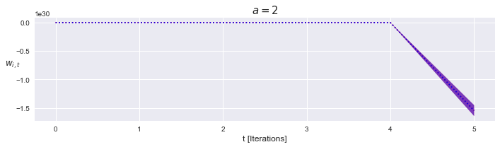
$\alpha> 0$, unstable

From the definition of $A$, if $\alpha > 0$ the system diverges exponentially.

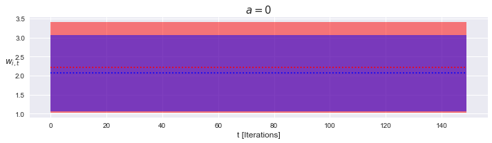
$\alpha = 0$, stable

In this case, the weights should diverge linearly. However, because $\beta_{i,1}$ depends on $\alpha$ and $\beta_{i1}$ is also the constant multiple in the geometric series, the sum itself vanishes and the trajectory is stationary.

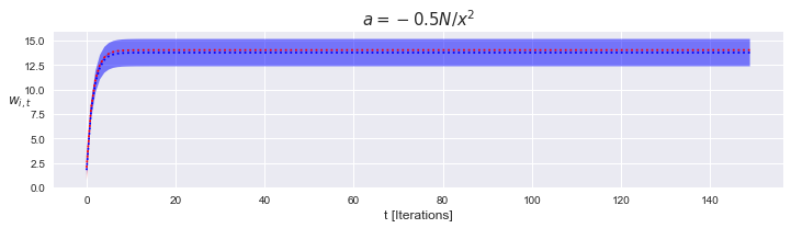
$-\frac{N}{|\mathbf{x}_i|} < \alpha < 0$, stable

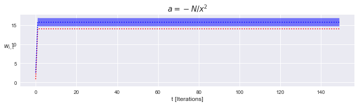
$\alpha = -\frac{N}{|\mathbf{x}_i|^2}$, stable.

Plugging this into (24) yields an expression

$$w_t = 0^t\left(w_0 + \frac{\mathbf{x}_i\cdot\mathbf{y}}{\|\mathbf{x}_i\|^2}\right)+\frac{\mathbf{x}_i\cdot\mathbf{y}}{\|\mathbf{x}_i\|^2}$$

This is actually interesting because the system converges in one iteration. The first term vanishes for $t>0$, such that the closed form solution is $\frac{\mathbf{x}_i\cdot\mathbf{y}}{|\mathbf{x}_i|^2}$

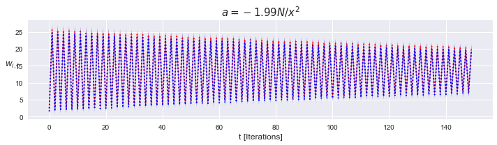
$\lim\limits_{k \to -2^+} \alpha = -k\frac{N}{|\mathbf{x}_i|}$, stable

Recall from the definiton of $A$ that its left bound is open. As such, the dynamics of learning are convergent for values of $\alpha$ infinitesimally close to $2$.

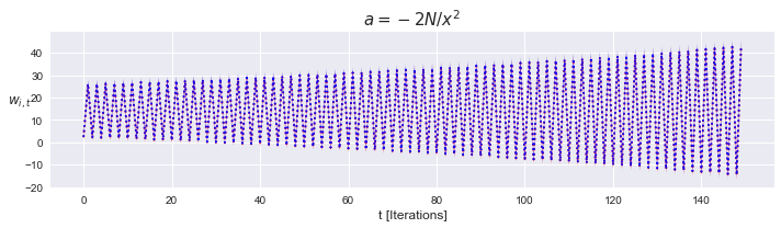
$\alpha = -2\frac{N}{|\mathbf{x}_i|^2}$, stable

By plugging in this value of $\alpha$, we get an oscillator.

$$w_t =(-1)^t w_0 + \frac{\mathbf{x}_i \cdot \mathbf{y}}{\|\mathbf{x}_i\|^2}\left((-1)^t -1\right)$$

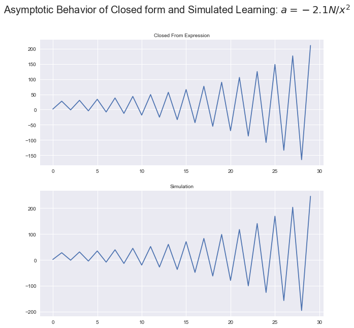
$\alpha > -2\frac{N}{|\mathbf{x}_i|^2}$, unstable

This time, we get a divergent oscillator

$$w_t =(-1)^t w_0 + \frac{\mathbf{x}_i \cdot \mathbf{y}}{\|\mathbf{x}_i\|^2}\left((-1)^t(1+ \epsilon)^t-1\right)$$

By neglecting the terms with constant magnitude, we can rewrite (26) to emphasize its nature as a divergent oscillator.

$$w_t \propto \frac{\mathbf{x}_i \cdot \mathbf{y}}{\|\mathbf{x}_i\|^2}e^{i \pi t}e^{\ln{[1+\epsilon]}t}$$

If we look back at our work, (26) oscillates only because gradient descent looks for the direction of descent, which is the negative of the error gradient with respect to weights.

Polynomials

It is not hard to imagine cases where we write $\hat{y}$ as a linear combination of multivariate polynomials.

$$\hat{y} = \sum\limits_{i=0}^K\mathbf{w_i}\left(\mathbf{x}^{T}\right)^j$$

While at first glance this seems nasty, it is actually not very different from the case of linear regression. This is because $\hat{y}$ remains a linear function of the weights; we have merely added $N\times(K-1)$ features to the dataset corresponding to $K$ powers of $N$ input variables. Thus, the analytical machinery we have developed extends to arbitrary polynomials. This is potentially useful because any function can be expressed as a polynomial.

Nonlinear Functions

Suppose we add a nonlinearity to the above polynomial system:

$$\hat{y} = \sigma\left( \sum\limits_{i=1}^N\sum\limits^{K}_{j=0} w_{ij}x_i^j\right)$$

This is actually surprisingly easy to fit if we use $y^\prime= \sigma^{-1}(y)$ as the dependent variable instead of just $y$. This effectively unrolls the nonlinearity so all the work involves a linear system, which means the analytics we have studied still apply.

Dynamical Bifurcations

At this point we have identified some significant $\alpha$ values and studied the dynamics of the system under such values. To review, we observed stationary dynamics for $\alpha=0$, logistic growth or decay for $\alpha = -N/{| x |^2}$, and oscillatory divergence for $\alpha = -2N/{|x|^2}$. Now, notice our equations are continuous for all values of $\alpha$. Thus, with equation (24) we can continuously interpolate between these the distinct dynamical regimes.

The boundary points of the set $A$ are dynamical bifurcation points. Suppose the boundary points of $A$ are used to dissect the real line into disjoint subsets. The qualitative behavior of learning dynamics is distinct for values of $\alpha$ picked from each of these subsets.

Discussion

We have derived exact analytical bounds on $\alpha$ values which lead to learning convergence and used these bounds to show analytically and computationaly the existence of distinct dynamical regimes in the learning dynamics of gradient descent in linear least squares regression. As the alpha parameter is varied, the system travels through different modes of stability but is always stable at the true weight value. Through some auxilary calculations revealed exponentially small convergence timescales. Lastly, we showed that these results also hold for nonlinear and polynomial regression.

This article is only a basic preview of what is to come. The presentation here is limited to instances where the Gaussian noise assumption can be made. It doesn’t consider alternative error functions. The analysis is restricted to the deterministic but in the future could include comments (1) on how the learning is affected by the spatial distribution of the independent variables and (2) on initial weight conditions.

Although linear regression has a closed form solution, that such analytical results on the dynamics of gradient descent is exciting. It shows that understanding the learning behavior of gradient descent dynamical systems is actually quite a tractable problem. This ought to inspire efforts to understand the learning process of more complex optimization tasks. This is practically useful as with deeper understanding comes more powerful algorithms. In the longer run, it will be extremely valuable to the effort to decipher the fundamental algorithms underlying intelligent, learning, systems.

Supplementary Materials

The code used to generate the figures can be found here